Primer on symplecticity#
Symplectic condition#
Hamiltonian equation in matrix form#
For a N-dimensional Hamiltonian system (\(\mathbf{x}^N, \mathbf{p}^N\)), the N sets of Hamiltonian equation reads:
Let’s write a column vector \(X=(x_1, p_1, x_2,p_2,\cdots,x_N,p_n)\), the Hamiltonian can be written as:
where \(S_1\) is the matrix for one dimension space:
Properties of S matrix#
We found that the following facts about \(S\) matrix
Determinant: \(\left|S\right|=1\)
Inverse: \(S^{-1}=-S \text{ or } S^2 = -I\)
The transpose: \(S^T=-S\)
For arbitrary 2 by 2 matrix \(A\) we may prove that:
Or we may define a new matrix \(\bar{A}=-S_2A^{T}S_2\) and yield:
Symplectic condition#
For a map from location \(s_0\) to \(s_1=s_0+s\), we have:
M is a matrix and the components is defined as:
If \(M_{ij}\) are not functions of \(X\), the map represents a linear map. Otherwise \(M\) is a non-linear map. Regardless of the linearity, the condition that map \(M\) need to follow due to the system is a Hamiltonian system is called symplectic condition. We just explored the condition in 1-D case. In N-D system, from the Map definition:
We take the derivative of the \(i^{th}\) row of \(X(s_1)\) with respect to \(s\):
We know that
Therefore we have
Using the property of \(S\), we have the usual form:
The equation (12) is referred as symplectic condition of a transfer map (not limited to matrix).
Properties of symplectic map#
The properties of the symplectic map:
If \(M\) is symplectic, so does \(M^T\) and \(M^{-1}\).
If \(M\) and \(N\) are symplectic, so does \(MN\).
The determinant of symplectic map is 1.
Properties of symplectic matrix#
The symplectic matrix has the following properties from the symplectic condition:
If \(\lambda\) is an eigenvalue of a symplectic matrix \(M\), so does \(1/\lambda\).
Every sympletic matrix has the inverse matrix: \(M^{-1}=-SM^{T}S\)
Block matrix for 2-D system#
Consider a 4-D phase space transfer map:
The transfer map has to satisfy the symplectic condition, both \(M^TSM=S\) and \(MSM^T=S\). For the first condition:
Show code cell content
import sympy
sympy.init_printing(use_unicode=True)
a=sympy.MatrixSymbol('A', 2,2)
b=sympy.MatrixSymbol('B', 2,2)
c=sympy.MatrixSymbol('C', 2,2)
d=sympy.MatrixSymbol('D', 2,2)
s_2=sympy.MatrixSymbol('S_2', 2,2)
zero=sympy.ZeroMatrix(2,2)
M=sympy.BlockMatrix([[a,b],[c,d]])
ss=sympy.BlockMatrix([[s_2,zero],[zero,s_2]])
sympy.block_collapse(M.T*ss*M)
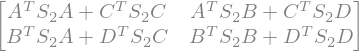
Therefore the following relation satisfy:
Change \(M\) to \(M^T\), we have
From the general property of 2-by-2 matrix \(A\):
From the first set equations in (16) and (17), we know that:
Or it can be re-written as:
And from second set equations in (16) and (17), we have
Note
It is worthwhile to note that, the symplectic condition for 4-D matrix (Eq. (19) and (21)) seems to have 9 equations on the coordinates. However, the actual constrains for 4-D are only 6.
The inverse of a blocked 4-by-4 matrix is simply:
Here is a useful example. If we are exploring \(x\)-\(z\) or \(y\)-\(z\) phase space, the matrix \(U\) usually has the form below for DC magnets:
Then
And from
We have
Block matrix for 3-D system#
Consider a 6-D phase space transfer map:
Show code cell content
import sympy
sympy.init_printing(use_unicode=True)
m1=sympy.MatrixSymbol('M_1', 2,2)
m2=sympy.MatrixSymbol('M_2', 2,2)
m3=sympy.MatrixSymbol('M_3', 2,2)
u1=sympy.MatrixSymbol('U_1', 2,2)
u2=sympy.MatrixSymbol('U_2', 2,2)
c1=sympy.MatrixSymbol('C_1', 2,2)
v1=sympy.MatrixSymbol('V_1', 2,2)
v2=sympy.MatrixSymbol('V_2', 2,2)
c2=sympy.MatrixSymbol('C_2', 2,2)

s_2=sympy.MatrixSymbol('S_2', 2,2)
#s_2=sympy.Matrix([[0,1],[-1,0]])
zero=sympy.ZeroMatrix(2,2)
M=sympy.BlockMatrix([[m1,c1,u1],[c2,m2,u2],[v1,v2,m3]])
ss=sympy.BlockMatrix([[s_2,zero,zero],[zero,s_2,zero],[zero,zero,s_2]])
sympy.block_collapse(M*ss*M.T)

Therefore, we can get the relation of the determinant of each block:
and
From the off diagonal blocks we have: